![]()
Package ‘ggpmisc’ (Miscellaneous Extensions to ‘ggplot2’) is a set of extensions to R package ‘ggplot2’ (>= 3.0.0) with emphasis on annotations and plotting related to fitted models. Estimates from model fit objects can be displayed in ggplots as text, tables or equations. Predicted values, residuals, deviations and weights can be plotted for various model fit functions. Linear models, quantile regression and major axis regression as well as those functions with accessors following the syntax of package ‘broom’ are supported. Package ‘ggpmisc’ continues to give access to extensions moved as of version 0.4.0 to package ‘ggpp’.
Statistics that help with reporting the results of model fits are:
| Statistic |
after_stat values (default geometry)
|
Methods |
|---|---|---|
stat_poly_eq()
|
equation, R2, P, etc. (text_npc)
|
lm, rlm (weight aesthetic fully supported) |
stat_ma_eq()
|
equation, R2, P, etc. (text_npc)
|
lmodel2: MA, SMA, RMA, OLS |
stat_quant_eq()
|
equation, P, etc. (text_npc)
|
rq (any number of quantiles) |
stat_correlation()
|
correlation, P-value, CI (
text_npc)
|
Pearson (t), Kendall (z), Spearman (S)
|
stat_poly_line()
|
line + conf. (smooth)
|
lm, rlm (weight aesthetic fully supported) |
stat_ma_line()
|
line + conf. (smooth)
|
lmodel2: MA, SMA, RMA, OLS |
stat_quant_line()
|
line + conf. (smooth)
|
rq, rqss (any number of quantiles) |
stat_quant_band()
|
median + quartiles (smooth)
|
rq, rqss (two or three quantiles) |
stat_fit_residuals()
|
residuals (point)
|
lm, rlm (weight aesthetic fully supported) |
stat_fit_deviations()
|
deviations from observations (segment)
|
lm, rlm (weight aesthetic fully supported) |
stat_fit_glance()
|
equation, R2, P, etc. (text_npc)
|
all those supported by ‘broom’ |
stat_fit_augment()
|
predicted and other values (smooth)
|
all those supported by ‘broom’ |
stat_fit_tidy()
|
fit results, e.g., for equation (text_npc)
|
all those supported by ‘broom’ |
stat_fit_tb()
|
ANOVA and summary tables (table_npc)
|
all those supported by ‘broom’ |
Statistics stat_peaks() and stat_valleys() can be used to highlight and/or label maxima and minima in a plot.
Scales scale_x_logFC() and scale_y_logFC() are suitable for plotting of log fold change data. Scales scale_x_Pvalue(), scale_y_Pvalue(), scale_x_FDR() and scale_y_FDR() are suitable for plotting p-values and adjusted p-values or false discovery rate (FDR). Default arguments are suitable for volcano and quadrant plots as used for transcriptomics, metabolomics and similar data.
Scales scale_colour_outcome(), scale_fill_outcome() and scale_shape_outcome() and functions outome2factor(), threshold2factor(), xy_outcomes2factor() and xy_thresholds2factor() used together make it easy to map ternary numeric outputs and logical binary outcomes to color, fill and shape aesthetics. Default arguments are suitable for volcano, quadrant and other plots as used for genomics, metabolomics and similar data.
Several geoms and other extensions formerly included in package ‘ggpmisc’ until version 0.3.9 were migrated to package ‘ggpp’. They are still available when ‘ggpmisc’ is loaded, but the documentation now resides in the new package ‘ggpp’.
![]()
Functions for the manipulation of layers in ggplot objects, together with statistics and geometries useful for debugging extensions to package ‘ggplot2’, included in package ‘ggpmisc’ until version 0.2.17 are now in package ‘gginnards’.
![]()
In the first example we plot a time series using the specialized version of ggplot() that converts the time series into a tibble and maps the x and y aesthetics automatically. We also highlight and label the peaks using stat_peaks.
ggplot(lynx, as.numeric = FALSE) + geom_line() +
  stat_peaks(colour = "red") +
  stat_peaks(geom = "text", colour = "red", angle = 66,
             hjust = -0.1, x.label.fmt = "%Y") +
  stat_peaks(geom = "rug", colour = "red", sides = "b") +
  expand_limits(y = 8000)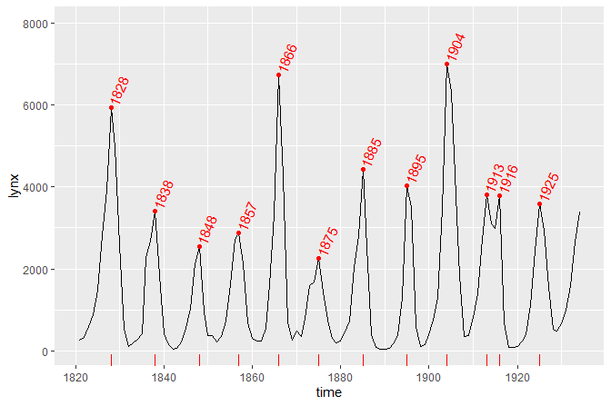
In the second example we add the equation for a fitted polynomial plus the adjusted coefficient of determination to a plot showing the observations plus the fitted curve, deviations and confidence band. We use stat_poly_eq().
formula <- y ~ x + I(x^2)
ggplot(cars, aes(speed, dist)) +
  geom_point() +
  stat_fit_deviations(formula = formula, colour = "red") +
  stat_poly_line(formula = formula) +
  stat_poly_eq(aes(label =  paste(stat(eq.label), stat(adj.rr.label), sep = "*\", \"*")),
               formula = formula)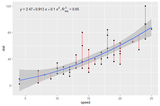
The same figure as in the second example but this time annotated with the ANOVA table for the model fit. We use stat_fit_tb() which can be used to add ANOVA or summary tables.
formula <- y ~ x + I(x^2)
ggplot(cars, aes(speed, dist)) +
  geom_point() +
  geom_smooth(method = "lm", formula = formula) +
  stat_fit_tb(method = "lm",
              method.args = list(formula = formula),
              tb.type = "fit.anova",
              tb.vars = c(Effect = "term",
                          "df",
                          "M.S." = "meansq",
                          "italic(F)" = "statistic",
                          "italic(P)" = "p.value"),
              tb.params = c(x = 1, "x^2" = 2),
              label.y.npc = "top", label.x.npc = "left",
              size = 2.5,
              parse = TRUE)
#> Dropping params/terms (rows) from table!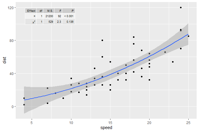
The same figure as in the second example but this time using quantile regression, median in this example.
formula <- y ~ x + I(x^2)
ggplot(cars, aes(speed, dist)) +
  geom_point() +
  stat_quant_line(formula = formula, quantiles = 0.5) +
  stat_quant_eq(aes(label = paste(stat(grp.label), stat(eq.label), sep = "*\": \"*")),
               formula = formula, quantiles = 0.5)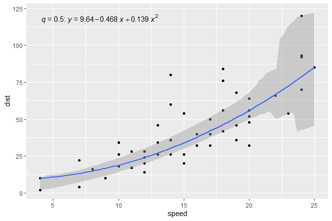
Band highlighting the region between both quartile regressions and a line for the median regression.
formula <- y ~ x + I(x^2)
ggplot(cars, aes(speed, dist)) +
  geom_point() +
  stat_quant_band(formula = formula)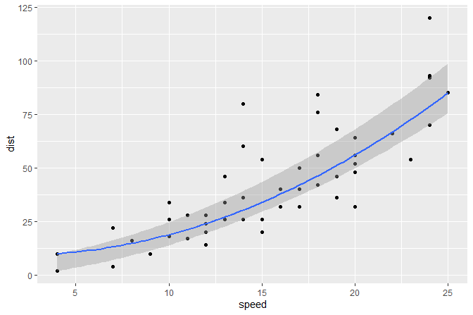
A quadrant plot with counts and labels, using geom_text_repel() from package ‘ggrepel’.
ggplot(quadrant_example.df, aes(logFC.x, logFC.y)) +
  geom_point(alpha = 0.3) +
  geom_quadrant_lines() +
  stat_quadrant_counts() +
  stat_dens2d_filter(color = "red", keep.fraction = 0.02) +
  stat_dens2d_labels(aes(label = gene), keep.fraction = 0.02,
                     geom = "text_repel", size = 2, colour = "red") +
  scale_x_logFC(name = "Transcript abundance after A%unit") +
  scale_y_logFC(name = "Transcript abundance after B%unit")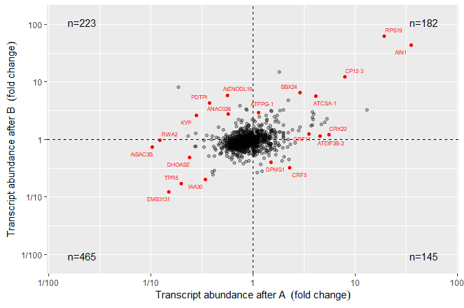
Installation of the most recent stable version from CRAN:
Installation of the current unstable version from GitHub:
HTML documentation for the package, including help pages and the User Guide, is available at https://docs.r4photobiology.info/ggpmisc/.
News about updates are regularly posted at https://www.r4photobiology.info/.
Chapter 7 in Aphalo (2020) explains basic concepts of the grammar of graphics as implemented in ‘ggplot2’ as well as extensions to this grammar including several of those made available by packages ‘ggpp’ and ‘ggpmisc’. Open access supplementary chapters and other information related to the book is available at https://www.learnr-book.info/.
Please report bugs and request new features at https://github.com/aphalo/ggpmisc/issues. Pull requests are welcome at https://github.com/aphalo/ggpmisc.
If you use this package to produce scientific or commercial publications, please cite according to:
citation("ggpmisc")
#>
#> To cite package 'ggpmisc' in publications use:
#>
#>   Pedro J. Aphalo (2022). ggpmisc: Miscellaneous Extensions to
#>   'ggplot2'. https://docs.r4photobiology.info/ggpmisc/,
#>   https://github.com/aphalo/ggpmisc.
#>
#> A BibTeX entry for LaTeX users is
#>
#>   @Manual{,
#>     title = {ggpmisc: Miscellaneous Extensions to 'ggplot2'},
#>     author = {Pedro J. Aphalo},
#>     year = {2022},
#>     note = {https://docs.r4photobiology.info/ggpmisc/,
#> https://github.com/aphalo/ggpmisc},
#> }Aphalo, Pedro J. (2020) Learn R: As a Language. The R Series. Boca Raton and London: Chapman and Hall/CRC Press. ISBN: 978-0-367-18253-3. 350 pp.
© 2016-2021 Pedro J. Aphalo (pedro.aphalo@helsinki.fi). Released under the GPL, version 2 or greater. This software carries no warranty of any kind.