modelsummary

modelsummary creates tables and plots to summarize statistical models and data in R.

The tables and plots produced by modelsummary are beautiful and highly customizable. They can be echoed to the R console or displayed in the RStudio Viewer. They can be saved to a wide variety of formats, including HTML, PDF, Text/Markdown, LaTeX, MS Word, RTF, JPG, and PNG. Tables can easily be embedded in dynamic documents with Rmarkdown, knitr, or Sweave. modelsummary supports hundreds of model types out-of-the-box. The look of your tables is infinitely customizable using external package such as kableExtra, gt, flextable, or huxtable.

modelsummary includes two families of functions:

Model Summary
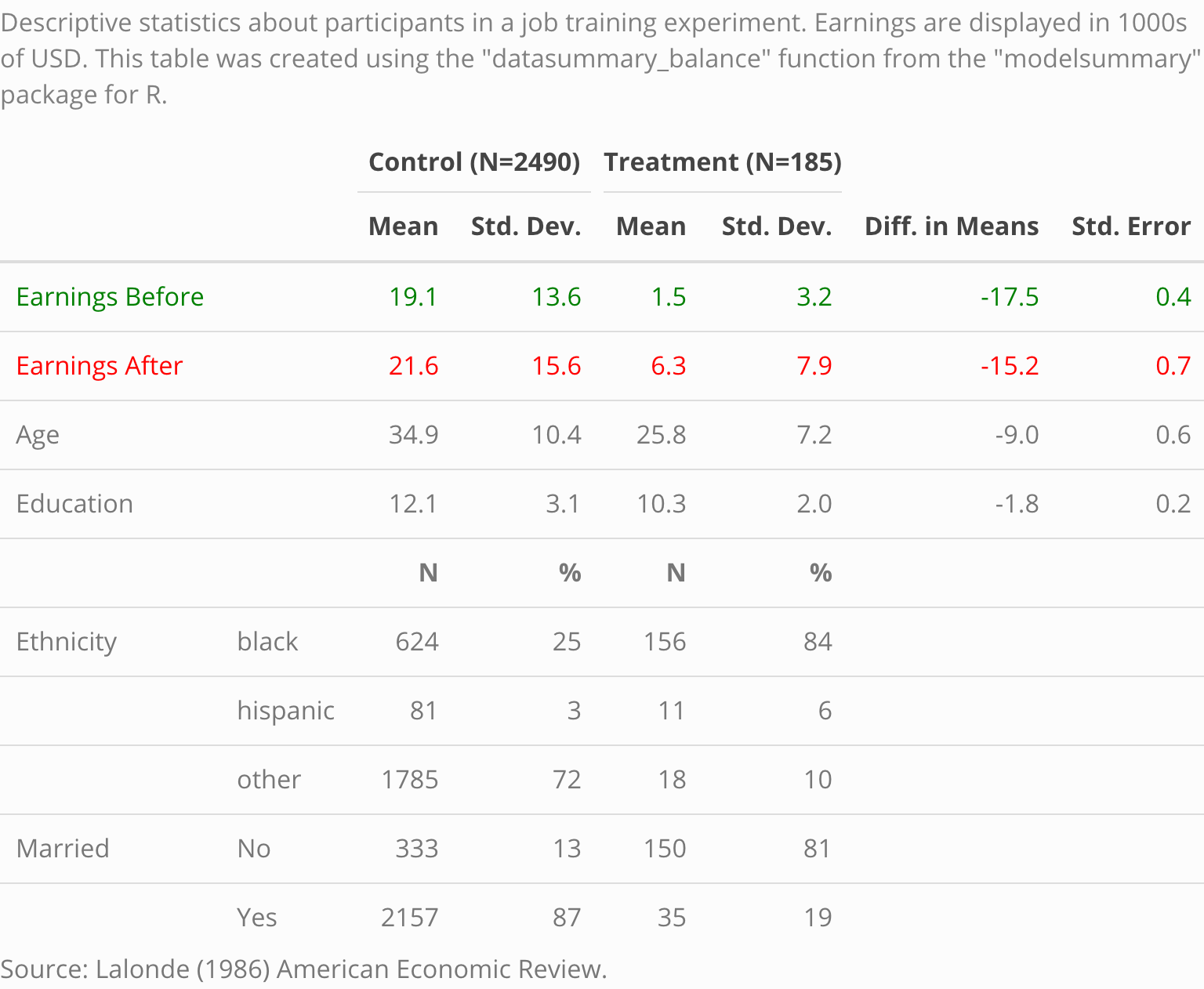
- modelsummary: Regression tables with side-by-side models.
- modelplot: Coefficient plots.
Data Summary
- datasummary: Powerful tool to create (multi-level) cross-tabs and data summaries.
- datasummary_crosstab: Cross-tabulations.
- datasummary_balance: Balance tables with subgroup statistics and difference in means (aka “Table 1”).
- datasummary_correlation: Correlation tables.
- datasummary_skim: Quick overview (“skim”) of a dataset.
- datasummary_df: Turn dataframes into nice tables with titles, notes, etc.

The modelsummary website hosts a ton of examples. Make sure you click on the links at the top of this page: https://vincentarelbundock.github.io/modelsummary

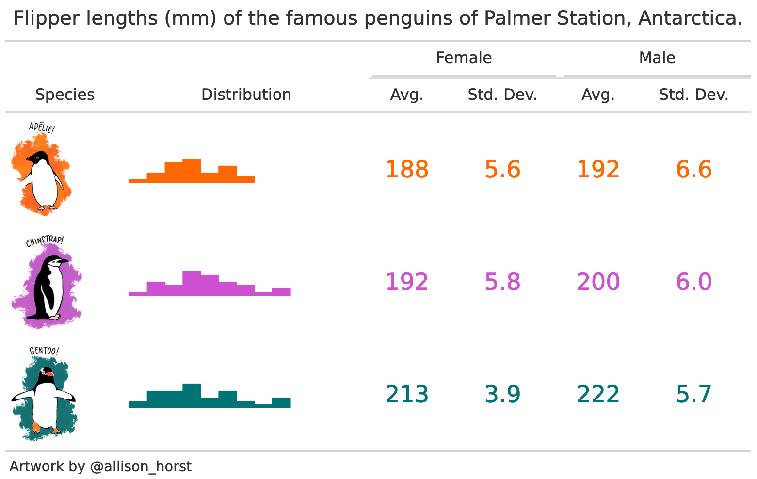
The following tables and plots were created using modelsummary, without any manual editing at all:

Why should I use `modelsummary`?

Here are a few benefits of modelsummary over some alternative packages:

Easy

modelsummary is very easy to use. This simple call often suffices:

library(modelsummary)

mod <- lm(y ~ x, dat)
modelsummary(mod)

The command above will automatically display a summary table in the Rstudio Viewer or in a web browser. All you need is one word to change the output format. For example, a text-only version of the table can be printed to the Console by typing:

modelsummary(mod, output = "markdown")

Tables in Microsoft Word and LaTeX formats can be saved to file by typing:

modelsummary(mod, output = "table.docx")
modelsummary(mod, output = "table.tex")

Flexible

Information: The package offers many intuitive and powerful utilities to customize the information reported in a summary table. You can rename, reorder, subset or omit parameter estimates; choose the set of goodness-of-fit statistics to include; display various “robust” standard errors or confidence intervals; add titles, footnotes, or source notes; insert stars or custom characters to indicate levels of statistical significance; or add rows with supplemental information about your models.

Appearance: Thanks to the gt, kableExtra, huxtable, and flextable packages, the appearance of modelsummary tables is endlessly customizable. The appearance customization page shows tables with colored cells, weird text, spanning column labels, row groups, titles, source notes, footnotes, significance stars, and more. This only scratches the surface of possibilities.

Supported models: Thanks to the broom and parameters, modelsummary supports hundreds of statistical models out-of-the-box. Installing other packages can extend the capabilities further (e.g., broom.mixed). It is also very easy to add or customize your own models.

Output formats: modelsummary tables can be saved to HTML, LaTeX, Text/Markdown, Microsoft Word, Powerpoint, RTF, JPG, or PNG formats. They can also be inserted seamlessly in Rmarkdown documents to produce automated documents and reports in PDF, HTML, RTF, or Microsoft Word formats.

Dangerous

modelsummary is dangerous! It allows users to do stupid stuff like replacing their intercepts by squirrels.

Reliable

modelsummary is reliably dangerous! The package is developed using a suite of unit tests with about 95% coverage, so it (probably) won’t break.

Community

modelsummary does not try to do everything. Instead, it leverages the incredible work of the R community. By building on top of the broom and parameters packages, modelsummary already supports hundreds of model types out-of-the-box. modelsummary also supports four of the most popular table-building and customization packages: gt, kableExtra, huxtable, and flextable. packages. By using those packages, modelsummary allows users to produce beautiful, endlessly customizable tables in a wide variety of formats, including HTML, PDF, LaTeX, Markdown, and MS Word.

One benefit of this community-focused approach is that when external packages improve, modelsummary improves as well. Another benefit is that leveraging external packages allows modelsummary to have a massively simplified codebase (relative to other similar packages). This should improve long term code maintainability, and allow contributors to participate through GitHub.

Installation

You can install modelsummary from CRAN:

install.packages('modelsummary')

If you want the very latest version, install it from Github:

library(remotes)
remotes::install_github('vincentarelbundock/modelsummary')

Getting started

There are a million ways to customize the tables and plots produced by modelsummary. In this Getting Started section we will only scratch the surface. For details, see the vignettes:

modelsummary: https://vincentarelbundock.github.io/modelsummary/articles/modelsummary.html
modelplot: https://vincentarelbundock.github.io/modelsummary/articles/modelplot.html
datasummary: https://vincentarelbundock.github.io/modelsummary/articles/datasummary.html
Appearance: https://vincentarelbundock.github.io/modelsummary/articles/appearance.html

To begin, load the modelsummary package and download data from the Rdatasets archive:

library(modelsummary)

url <- 'https://vincentarelbundock.github.io/Rdatasets/csv/HistData/Guerry.csv'
dat <- read.csv(url) 
dat$Small <- dat$Pop1831 > median(dat$Pop1831)

Quick overview of the data:

datasummary_skim(dat)

Balance table (aka “Table 1”) with differences in means by subgroups:

datasummary_balance(~Small, dat)

Correlation table:

datasummary_correlation(dat)

Two variables and two statistics, nested in subgroups:

datasummary(Literacy + Commerce ~ Small * (mean + sd), dat)

Estimate a linear model and display the results:

mod <- lm(Donations ~ Crime_prop, data = dat)

modelsummary(mod)

Estimate five regression models, display the results side-by-side, and save them to a Microsoft Word document:

models <- list(
  "OLS 1"     = lm(Donations ~ Literacy + Clergy, data = dat),
  "Poisson 1" = glm(Donations ~ Literacy + Commerce, family = poisson, data = dat),
  "OLS 2"     = lm(Crime_pers ~ Literacy + Clergy, data = dat),
  "Poisson 2" = glm(Crime_pers ~ Literacy + Commerce, family = poisson, data = dat),
  "OLS 3"     = lm(Crime_prop ~ Literacy + Clergy, data = dat)
)

modelsummary(models, output = "table.docx")

Alternative packages

There are several excellent alternatives to draw model summary tables in R: