![]()
The multilateral package provides one key function, that is multilateral(). The user provides the necessary attributes of a dataset to calculate their choice of multilateral methods.
See vignette for further information.
For some specific index calculation methods this package has been heavily influenced by Graham White’s IndexNumR package.
See bottom for all index and splice methods.
library(multilateral)
library(ggplot2)

tpd_index <- multilateral(period = turvey$month,
                          id = turvey$commodity,
                          price = turvey$price,
                          quantity = turvey$quantity,
                          splice_method = "geomean",
                          window_length = 13,
                          index_method = "TPD")

plot <- ggplot(tpd_index$index)+geom_line(aes(x = period, y = index))+theme_bw()

print(plot)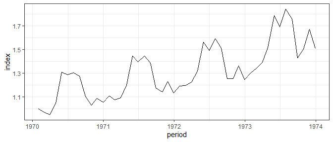
The function returns a list object containing
index: the continuous spliced index,index_windows: each individual window’s index,splice_detail: splicing information.str(tpd_index)
#> List of 3
#> $ index :Classes 'data.table' and 'data.frame': 48 obs. of 3 variables:
#> ..$ period : Date[1:48], format: "1970-01-31" "1970-02-28" ...
#> ..$ index : num [1:48] 1 0.971 0.949 1.047 1.308 ...
#> ..$ window_id: int [1:48] 1 1 1 1 1 1 1 1 1 1 ...
#> ..- attr(*, ".internal.selfref")=<externalptr>
#> $ index_windows:Classes 'data.table' and 'data.frame': 468 obs. of 3 variables:
#> ..$ period : Date[1:468], format: "1970-01-31" "1970-02-28" ...
#> ..$ index : num [1:468] 1 0.971 0.949 1.047 1.308 ...
#> ..$ window_id: int [1:468] 1 1 1 1 1 1 1 1 1 1 ...
#> ..- attr(*, ".internal.selfref")=<externalptr>
#> $ splice_detail:Classes 'data.table' and 'data.frame': 35 obs. of 5 variables:
#> ..$ period : Date[1:35], format: "1971-02-28" "1971-03-31" ...
#> ..$ latest_window_movement: num [1:35] 0.97 1.012 1.097 1.195 0.949 ...
#> ..$ revision_factor : num [1:35] 1 1 1 1.01 1.02 ...
#> ..$ update_factor : num [1:35] 0.972 1.013 1.099 1.205 0.966 ...
#> ..$ window_id : int [1:35] 2 3 4 5 6 7 8 9 10 11 ...
#> ..- attr(*, ".internal.selfref")=<externalptr>
#> - attr(*, "class")= chr [1:2] "list" "multilateral"
#> - attr(*, "params")=List of 6
#> ..$ index_method : chr "TPD"
#> ..$ window_length : num 13
#> ..$ splice_method : chr "geomean"
#> ..$ chain_method : NULL
#> ..$ check_inputs_ind: logi TRUE
#> ..$ matched : NULLThe index_windows returns all individual windows indexes before they were spliced. Below shows how you could (roughly) visualise this data
library(dplyr)
#> Warning: package 'dplyr' was built under R version 4.0.5
#>
#> Attaching package: 'dplyr'
#> The following objects are masked from 'package:stats':
#>
#>     filter, lag
#> The following objects are masked from 'package:base':
#>
#>     intersect, setdiff, setequal, union

#Get splice details to relevel each new index
update_factor <- tpd_index$splice_detail%>%
  mutate(update_factor  = cumprod(update_factor))%>%
  select(window_id, update_factor)


index_windows <- merge(tpd_index$index_windows,update_factor)

index_windows <-index_windows%>%mutate(updated_index = index*update_factor)
windows_plot <- ggplot(index_windows)+
  geom_line(aes(x = period, y = updated_index, group = window_id, colour = window_id))+
  theme_bw()

print(windows_plot)
splice_detail gives the user a break down of how the given periods index number is made up of both a ‘revision factor’ (from splicing) and the latest periods movement. This can be useful for diagnostics.
head(tpd_index$splice_detail)
#>        period latest_window_movement revision_factor update_factor window_id
#> 1: 1971-02-28              0.9698029        1.002095     0.9718351         2
#> 2: 1971-03-31              1.0120421        1.001120     1.0131760         3
#> 3: 1971-04-30              1.0973656        1.001151     1.0986290         4
#> 4: 1971-05-31              1.1950159        1.008111     1.2047081         5
#> 5: 1971-06-30              0.9490383        1.017805     0.9659356         6
#> 6: 1971-07-31              1.0336941        1.004028     1.0378582         7
Below shows one way in which you could visualise contribution of revision factor verses the latest movement.
library(dplyr)

#Period of interest
splice_detail <- tpd_index$splice_detail[period=="1973-02-28"]

#Log information to determine contribution
lwm_log <- log(splice_detail$latest_window_movement)
rf_log <- log(splice_detail$revision_factor)
sum_log <- sum(lwm_log+rf_log)

lwm_contrib <- lwm_log/sum_log
rf_contrib <- rf_log/sum_log


ggplot(mapping = aes(fill=c("Latest movement","Revision factor"),
                     y=c(lwm_contrib,rf_contrib),
                     x="1973-02-28"))+
  geom_bar(position="stack", stat="identity", width = 0.2)+
  theme_bw()+
  xlab("Date")+
  ylab("% Contribution")+
  labs(fill = "Contributor")+
  scale_fill_manual(values = c("#085c75","#d2ac2f"))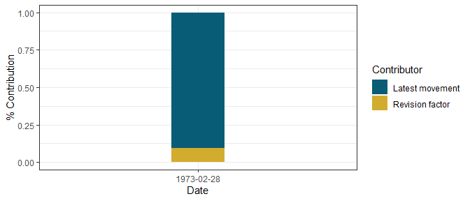
See vignette for further information.
|
Method |
Name |
Requires ID |
Requires Features |
Requires Quantity |
Requires Weight |
Can Restrict to Matched Sample |
|---|---|---|---|---|---|---|
|
TPD |
Time Product Dummy |
TRUE |
FALSE |
FALSE |
TRUE |
FALSE |
|
TDH |
Time Dummy Hedonic |
FALSE |
TRUE |
FALSE |
TRUE |
FALSE |
|
GEKS-J |
GEKS Jevons |
TRUE |
FALSE |
FALSE |
FALSE |
TRUE |
|
GEKS-T |
GEKS Tornqvist |
TRUE |
FALSE |
TRUE |
FALSE |
TRUE |
|
GEKS-F |
GEKS Fisher |
TRUE |
FALSE |
TRUE |
FALSE |
TRUE |
|
GEKS-IT |
GEKS Imputation Tornqvist |
TRUE |
TRUE |
TRUE |
FALSE |
TRUE |
|
splice_method |
|---|
|
geomean |
|
window |
|
movement |
|
geomean_short |
|
half |
|
chain_method |
|---|
|
geomean |
|
window |
|
movement |
|
half |