
![]()
rmweather is an R package to conduct meteorological/weather normalisation on air quality so trends and interventions can be investigated in a robust way. For those who are aware of my previous research, rmweather is the “Mk.II” package of normalweatherr. rmweather does less than normalweatherr, but it is much faster and easier to use.
rmweather is aviable from CRAN and can be installed in the normal way:
# Install rmweather from CRAN
install.packages("rmweather")To install the development version of rmweather, the devtools package will need to be installed first. Then:
# Load helper package
library(remotes)

# Install rmweather
install_github("skgrange/rmweather")rmweather contains example data from London which can be used to show the meteorological normalisation procedure. The example data are daily means of NO2 and NOx observations at London Marylebone Road. The accompanying surface meteorological data are from London Heathrow, a major airport located 23 km west of Central London.
Most of rmweather’s functions begin with rmw_ so are easy to track and find help for. In this example, we have used dplyr and the pipe (%>% and pronounced as “then”) for clarity. The example takes about a couple of minutes on my (laptop) system and the model has an R2 value of 77 %.
# Load packages
library(dplyr)
library(rmweather)
library(ranger)
# Have a look at rmweather's example data, from london
head(data_london)
# Prepare data for modelling
# Only use data with valid wind speeds, no2 will become the dependent variable
data_london_prepared <- data_london %>%
filter(!is.na(ws)) %>%
rename(value = no2) %>%
rmw_prepare_data(na.rm = TRUE)
# Grow/train a random forest model and then create a meteorological normalised trend
list_normalised <- rmw_do_all(
data_london_prepared,
variables = c(
"date_unix", "day_julian", "weekday", "air_temp", "rh", "wd", "ws",
"atmospheric_pressure"
),
n_trees = 300,
n_samples = 300,
verbose = TRUE
)
# What units are in the list?
names(list_normalised)
# Check model object's performance
rmw_model_statistics(list_normalised$model)
# Plot variable importances
list_normalised$model %>%
rmw_model_importance() %>%
rmw_plot_importance()
# Check if model has suffered from overfitting
rmw_predict_the_test_set(
model = list_normalised$model,
df = list_normalised$observations
) %>%
rmw_plot_test_prediction()
# How long did the process take?
list_normalised$elapsed_times
# Plot normalised trend
rmw_plot_normalised(list_normalised$normalised)
# Investigate partial dependencies, if variable is NA, predict all
data_pd <- rmw_partial_dependencies(
model = list_normalised$model,
df = list_normalised$observations,
variable = NA
)
# Plot partial dependencies
data_pd %>%
filter(variable != "date_unix") %>%
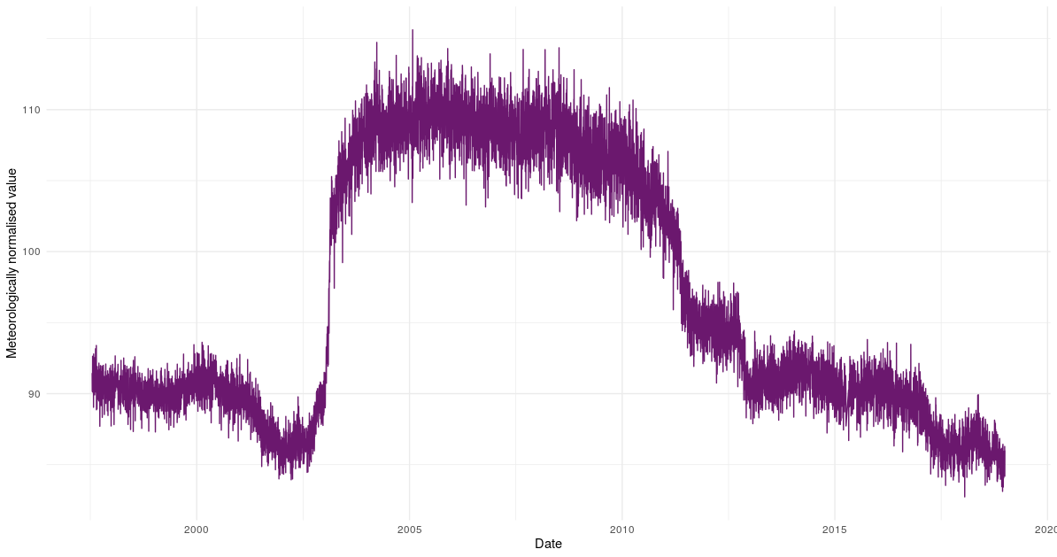
rmw_plot_partial_dependencies()The meteorologically normalised trend produced is below.
For usage examples see:
Grange, S. K., Carslaw, D. C., Lewis, A. C., Boleti, E., and Hueglin, C. (2018). Random forest meteorological normalisation models for Swiss PM10 trend analysis. Atmospheric Chemistry and Physics 18.9, pp. 6223–6239.
Grange, S. K. and Carslaw, D. C. (2019). Using meteorological normalisation to detect interventions in air quality time series. Science of The Total Environment 653, pp. 578–588.